Shiny tutorial
This tutorial walks you through the MCNV2 Shiny application with step-by-step instructions.
The Shiny app provides interactive Mendelian Precision exploration with real-time filtering, visualization, and export capabilities.
Launching the app
From R console:
library(reticulate)
use_virtualenv("r-MCNV2", required = TRUE)

library(MCNV2)
MCNV2::launch(
  bedtools_path = Sys.which("bedtools"),
  results_dir = "~/mcnv2_results"
)
Parameters:
bedtools_path — Path to bedtools executable (required for annotation)
results_dir — Directory to save output files (default: temporary directory)
The app will open in your default web browser.
—
Step 1: Preprocessing tab
The Preprocessing tab handles CNV annotation and inheritance calculation.
Upload files and set parameters
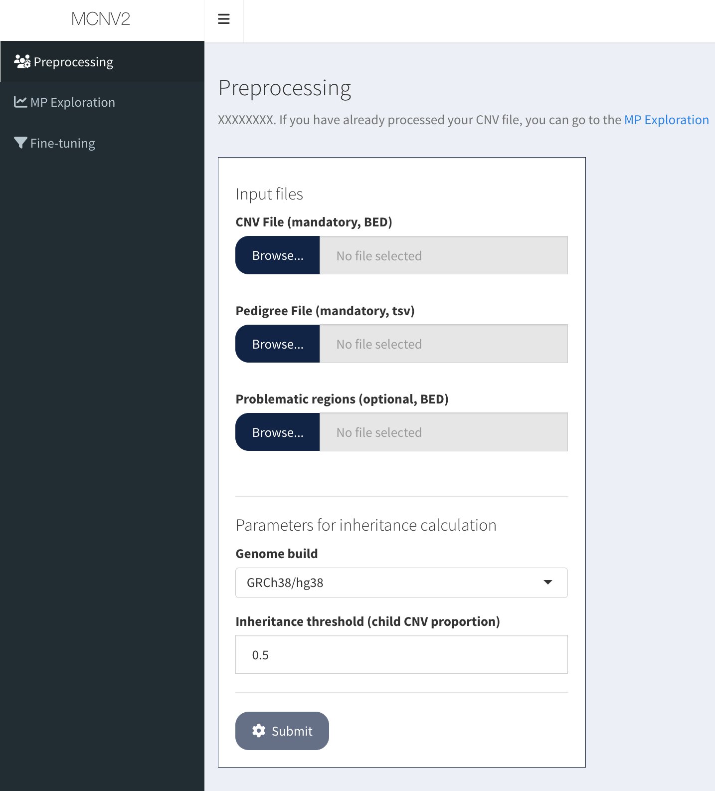
Input files panel with three file upload buttons and parameters section
Required files:
CNV file (tab-delimited) - Required columns: CHR, START, STOP, TYPE, SAMPLE_ID
Pedigree file (tab-delimited, no header) - Three columns: SAMPLE_ID, FATHER_ID, MOTHER_ID
Optional file:
Problematic regions (BED format) - Default file provided if not uploaded
Parameters:
Inheritance threshold: Minimum overlap for a CNV to be considered inherited (default: 0.5)
Genome build: GRCh38/hg38 or hg19
Upload workflow:
Click Browse next to each file type
Select your files
Set inheritance threshold (0.5 recommended)
Click Submit to start annotation
Input CNV file format
Your input CNV file should contain the required columns plus any optional quality metrics:
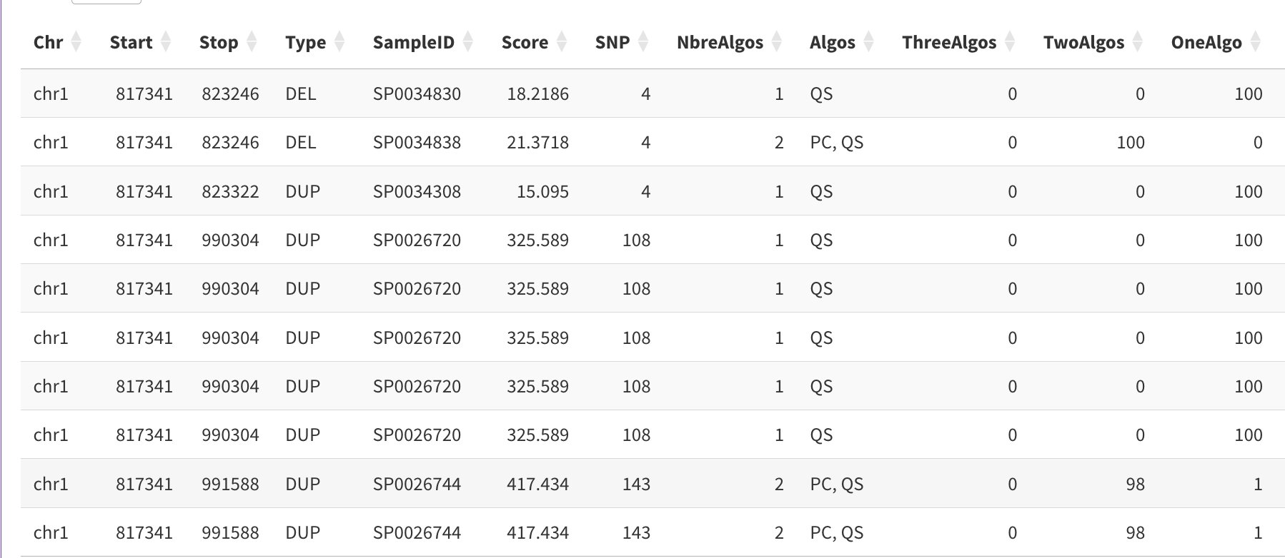
Example input CNV file showing required columns (Chr, Start, Stop, Type, SampleID) and optional quality columns (Score, SNP, NbreAlgos, Algos, ThreeAlgos, TwoAlgos, OneAlgo)
Column descriptions:
Chr, Start, Stop — CNV genomic coordinates (required)
Type — DEL or DUP (required)
SampleID — Sample identifier matching pedigree file (required)
Score — Quality score from CNV caller (optional)
SNP — Number of supporting probes (optional, array data)
NbreAlgos — Number of algorithms detecting the CNV (optional, merged callsets)
Algos — Algorithm names (optional, e.g., “PC, QS”)
ThreeAlgos, TwoAlgos, OneAlgo — Boolean flags for algorithm counts (optional)
Annotate CNVs
Click Submit to start annotation. The app will:
Intersect CNVs with gene coordinates (Gencode)
Add LOEUF constraint scores (gnomAD v4)
Calculate problematic region overlap
Output: Annotation table
The annotation process adds new columns to your CNV file:
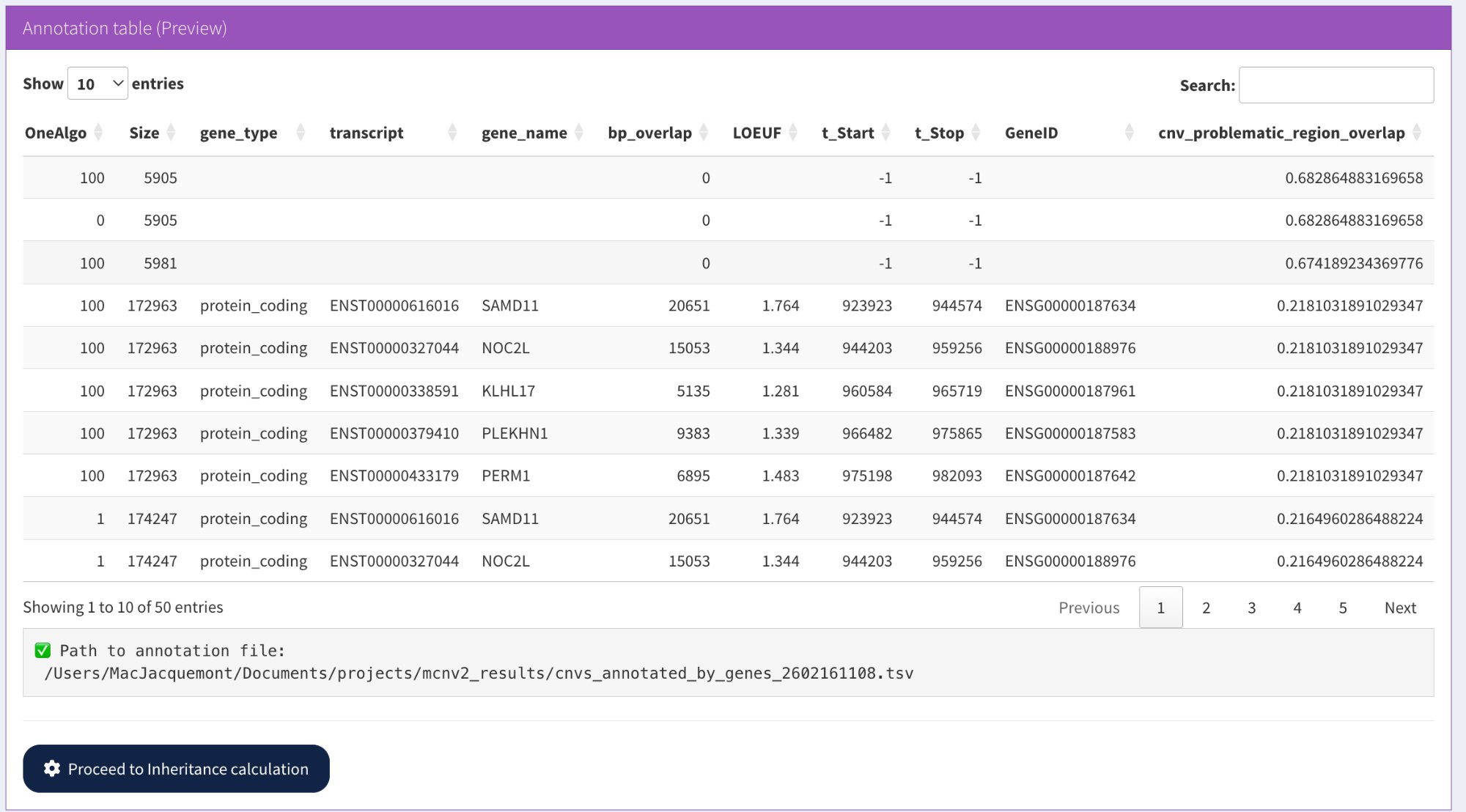
Columns added by annotation: gene information (gene_name, transcript, GeneID), constraint scores (LOEUF), and problematic region overlap percentage
New columns added:
Size — CNV size in bp (Stop - Start)
gene_type — Type of gene overlapped (e.g., protein_coding)
transcript — Ensembl transcript ID (e.g., ENST00000616016)
gene_name — HGNC gene symbol (e.g., SAMD11, NOC2L)
bp_overlap — Base pairs overlapping the gene
LOEUF — Loss-of-function constraint score (gnomAD v4)
t_Start, t_Stop — Transcript coordinates
GeneID — Ensembl gene ID (e.g., ENSG00000187634)
cnv_problematic_region_overlap — Percentage overlap with problematic regions
Note: If a CNV overlaps multiple genes, one row per gene is created. Intergenic CNVs have gene fields set to -1 or 0.
Compute inheritance status
Click Proceed to Inheritance calculation to calculate transmission status.
What happens:
CNV-level matching — Coordinate-based comparison (reciprocal overlap ≥ threshold)
Gene-level matching — Gene-based comparison (at least one shared gene)
See Inheritance status for detailed algorithm explanation.
Output: Inheritance table
The inheritance calculation adds transmission status columns:
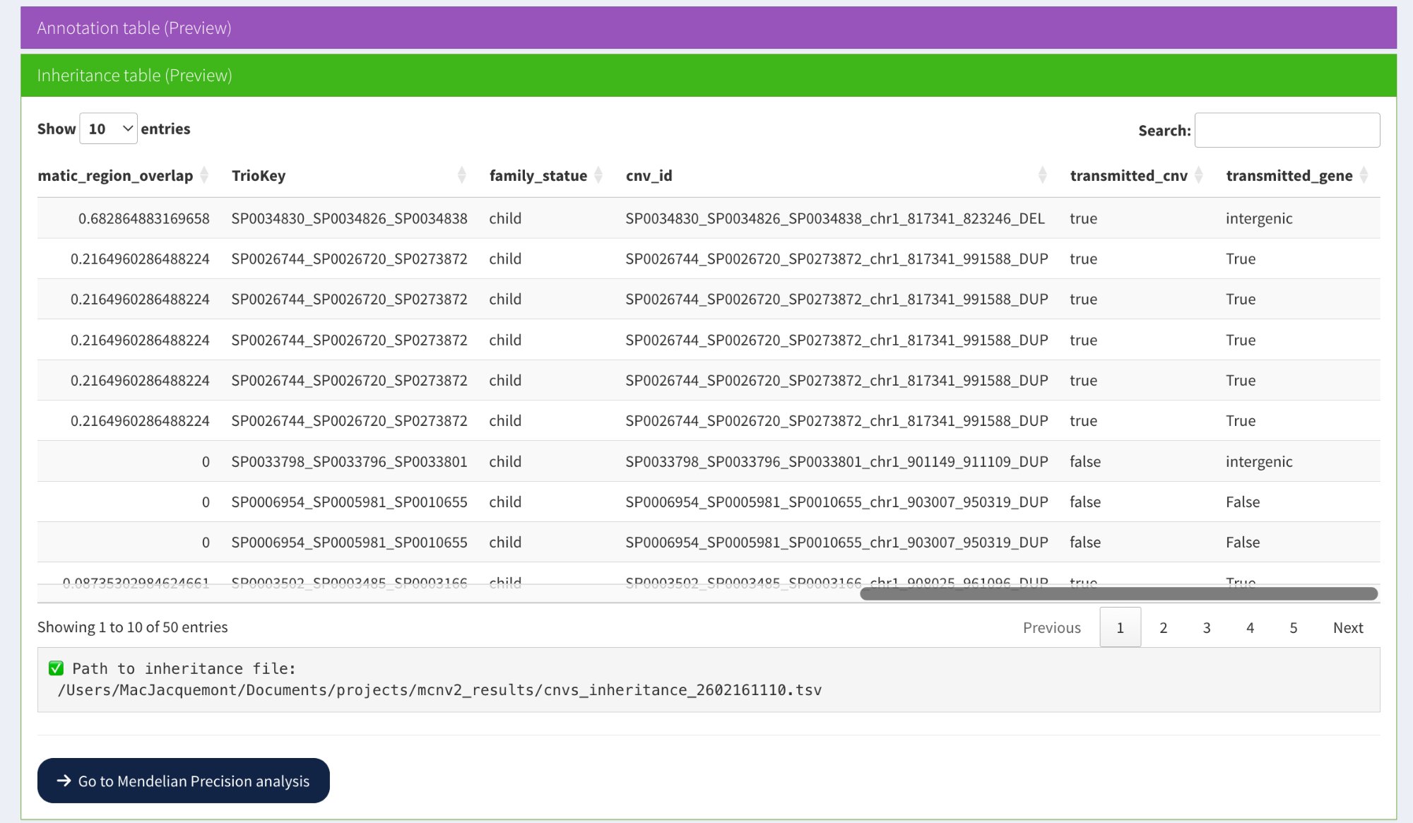
Key columns added: transmitted_cnv (true/false) and transmitted_gene (True/False/intergenic) showing inheritance status for each CNV
New columns added:
TrioKey — Trio identifier (father_mother_child sample IDs)
family_statue — Role in trio (typically “child”)
cnv_id — Unique CNV identifier
transmitted_cnv — Coordinate-based inheritance status:
true — CNV inherited from at least one parent
false — Candidate de novo CNV
transmitted_gene — Gene-based inheritance status:
True — At least one overlapping gene is inherited
False — No overlapping genes are inherited (candidate de novo)
intergenic — CNV does not overlap any genes
Interpretation examples from screenshot:
Row 1: transmitted_cnv=**true**, transmitted_gene=**intergenic** → Inherited CNV, no genes affected
Rows 2-6: transmitted_cnv=**true**, transmitted_gene=**True** → Inherited CNV and genes
Row 7: transmitted_cnv=**false**, transmitted_gene=**intergenic** → Candidate de novo, intergenic
Rows 8-9: transmitted_cnv=**false**, transmitted_gene=**False** → Candidate de novo, affecting genes
Next step:
Click Go to Mendelian Precision analysis to proceed to the MP Exploration tab where you can apply filters and visualize Mendelian Precision.
—
Step 2: MP Exploration tab
The MP Exploration tab provides interactive Mendelian Precision analysis with real-time filtering and visualization.
Interface overview and access methods
The MP Exploration tab can be accessed in two ways and provides comprehensive filtering options:
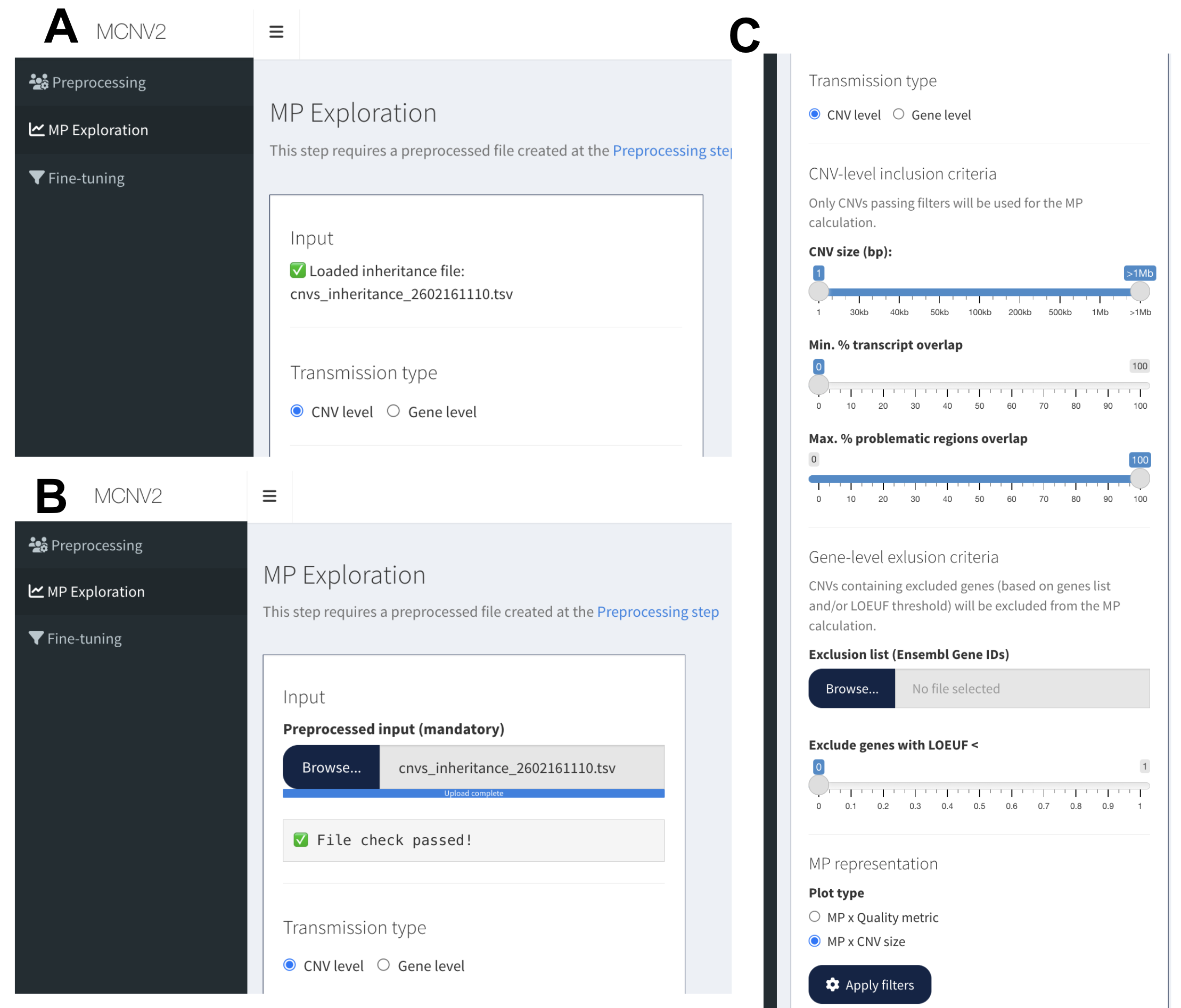
Panel A: Direct access via MP Exploration tab (file auto-loaded from Preprocessing). Panel B: Manual file upload when accessing tab directly. Panel C: Complete interface showing transmission type selection, CNV filtering criteria, gene exclusion options, and plot type selection.
Access methods:
Method 1 (Panel A): After Preprocessing, click Go to Mendelian Precision analysis → File automatically loaded
Method 2 (Panel B): Navigate directly to MP Exploration tab → Manual file upload required
Interface components (Panel C):
Transmission type: CNV level vs Gene level
CNV-level inclusion criteria: Size filters, transcript overlap, problematic regions
Gene-level exclusion criteria: Gene lists, LOEUF threshold
MP representation: Plot type selection (Size vs Quality metric)
Transmission type selection
Choose how inheritance is evaluated:
CNV level — Uses Transmitted_CNV (coordinate-based matching)
Gene level — Uses Transmitted_gene (gene-based matching)
When to use each:
CNV level: Evaluates transmission based on genomic coordinates (reciprocal overlap)
Gene level: Evaluates transmission based on shared genes between child and parents
See Inheritance status for detailed explanation of the two approaches.
Filtering criteria
Apply filters to focus the MP analysis. These filters are available regardless of transmission type (CNV level vs Gene level):
Size and overlap filters:
CNV size filter:
Slider range: 1 bp to >1 Mb
Use to filter out very small or very large CNVs
Example: Set minimum to 30 kb to focus on medium-large CNVs
Min. % transcript overlap:
Range: 0-100%
Minimum percentage of CNV overlapping a gene transcript
Useful to focus on genic CNVs (set to >0%)
Max. % problematic regions overlap:
Range: 0-100%
Maximum allowed overlap with problematic regions
Recommended: ≤50% to exclude low-confidence regions
Gene-based exclusion filters:
Exclusion list (Ensembl Gene IDs):
Upload a text file with one Ensembl Gene ID per line
CNVs overlapping these genes will be excluded from MP calculation
Use case: Exclude known highly polymorphic genes
Exclude genes with LOEUF <:
Slider range: 0-1
Excludes constrained genes (low LOEUF values)
Recommended: 0.6 to focus on technical MP (excluding likely de novo)
See Filtering strategies for LOEUF guidance
Note
CNV level vs Gene level affects only transmission evaluation. Both transmission modes can use the same filtering criteria because CNV annotation includes gene information regardless of how transmission is calculated.
MP representation
Choose the plot type to visualize:
MP x CNV size (default):
Bar plots showing MP for each size range
Separate plots for DEL and DUP
X-axis: 7 size bins (1-30kb, 30-50kb, 50-100kb, 100-200kb, 200-500kb, 500kb-1Mb, >1Mb)
Y-axis: Mendelian Precision (%)
Numbers on bars: CNV count (n)
MP x Quality metric:
Line plots showing MP vs quality score threshold
Separate plots for DEL and DUP
X-axis: Score threshold (≥)
Y-axis: Mendelian Precision (%)
Multiple lines: One per size range
Interactive tooltips: Hover to see MP, n, size range, threshold
Click Apply filters to generate the analysis.
Summary cards and filtered table
After applying filters, three summary cards display global statistics:
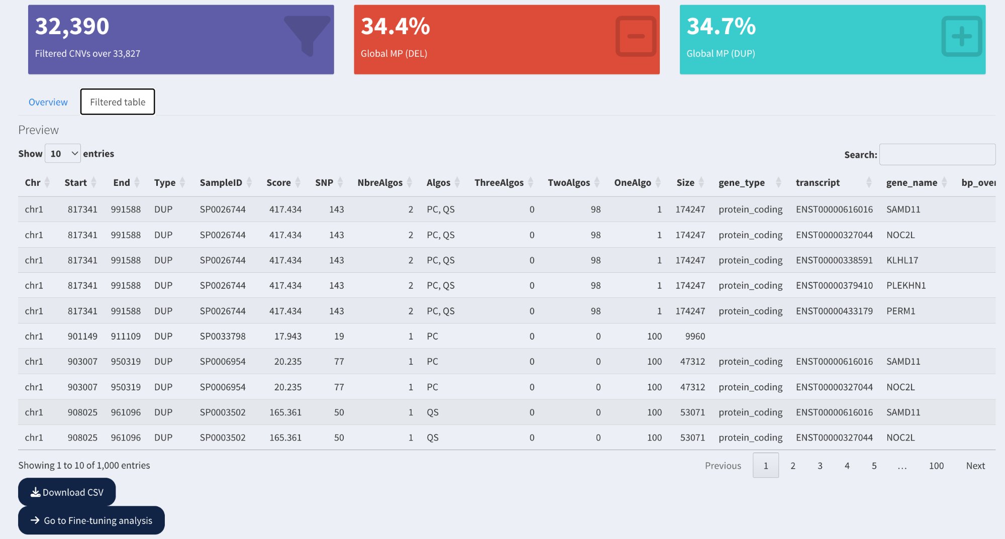
Summary cards showing total CNV count, Global MP (DEL), and Global MP (DUP), followed by the filtered CNV table with all annotation and inheritance columns.
Summary cards:
Purple card: Filtered CNV count (e.g., 32,390 CNVs passing filters out of 33,827 total)
Red card: Global Mendelian Precision for deletions (%)
Cyan card: Global Mendelian Precision for duplications (%)
Filtered table:
Overview tab: Summary statistics
Filtered table tab: Complete CNV table with all columns
Shows only CNVs passing the applied filters
Pagination: Navigate through results (10/50/100 entries per page)
Search: Use search box to find specific samples, genes, or coordinates
Download: Click Download CSV to export filtered CNVs
Action buttons:
Download CSV: Export filtered CNV table
Go to Fine-tuning analysis: Proceed to quality threshold optimization
MP by CNV size visualization
When MP x CNV size is selected, bar plots display MP for each size range:
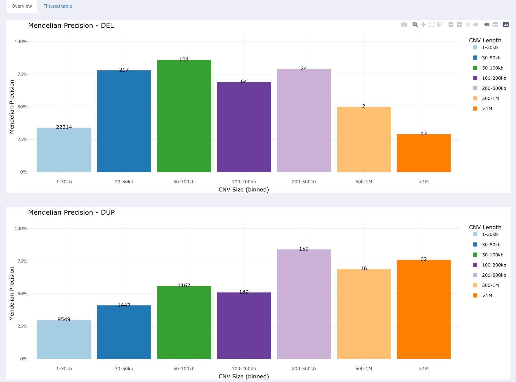
Bar plots showing Mendelian Precision for each size range, separately for deletions (top) and duplications (bottom). Numbers on bars indicate CNV count.
Plot features:
Two panels: Top = Deletions (DEL), Bottom = Duplications (DUP)
X-axis: 7 size ranges (1-30kb, 30-50kb, 50-100kb, 100-200kb, 200-500kb, 500kb-1Mb, >1Mb)
Y-axis: Mendelian Precision (0-100%)
Bar colors: Different color per size range (visual distinction)
Numbers on bars: CNV count (n) for that size range
Legend: Size ranges with color coding
Interpretation:
Low MP for small CNVs: 1-30kb typically shows lower MP (~30-35%)
Higher MP for large CNVs: >100kb typically shows higher MP (>75%)
Interactive features:
Hover over bars to see exact MP value
Toolbar icons: Zoom, pan, download PNG
Click plot title to open modal for enlarged view
MP by quality metric visualization
When MP x Quality metric is selected, line plots display MP vs score threshold:
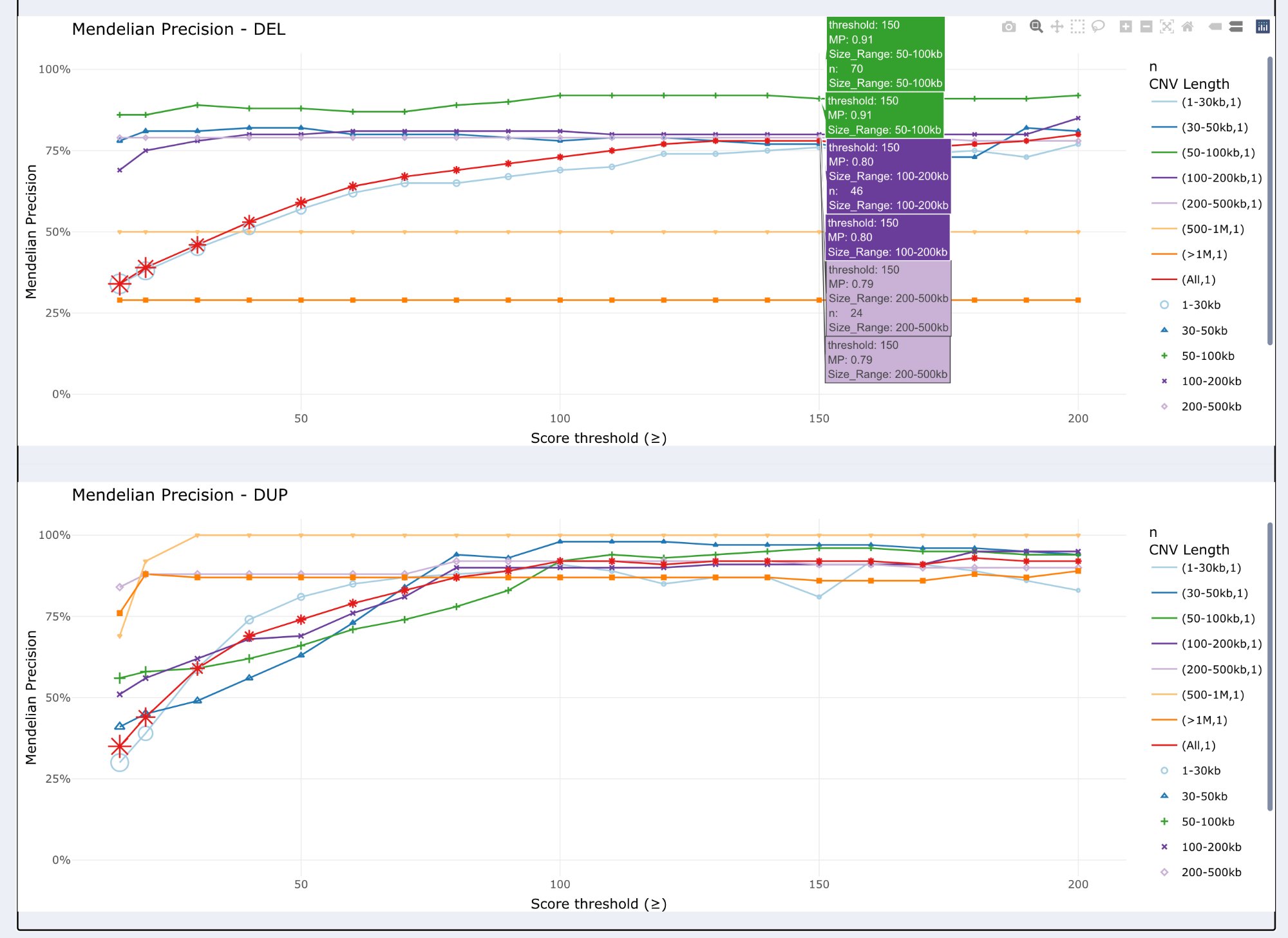
Line plots showing Mendelian Precision as a function of quality score threshold, separately for deletions (top) and duplications (bottom). Each line represents a different size range.
Plot features:
Two panels: Top = Deletions (DEL), Bottom = Duplications (DUP)
X-axis: Score threshold (≥ values from 0 to 200)
Y-axis: Mendelian Precision (0-100%)
Multiple lines: One line per size range (7 lines + “All” line) * 7 size-specific lines: 1-30kb, 30-50kb, 50-100kb, 100-200kb, 200-500kb, 500kb-1Mb, >1Mb * “All” line: All size ranges combined together
Line colors: Match size range colors from bar plots
Star markers: Indicate specific threshold points
Interactive tooltips: Hover to see detailed info (threshold, MP, n, size range)
Interpretation:
Trend observation: MP generally increases with higher score thresholds
Plateau identification: Look for where MP stops improving significantly
Size-specific patterns: Small CNVs (1-30kb) require higher thresholds for good MP
Trade-off assessment: Balance MP improvement vs CNV count loss
Next steps
From the MP Exploration tab, you can:
Download filtered CNVs: Click Download CSV to export the table
Refine analysis: Adjust filters and re-run to explore different scenarios
Proceed to Fine-tuning: Click Go to Fine-tuning analysis for systematic quality threshold optimization
—
Step 3: Fine-tuning tab
The Fine-tuning tab enables systematic optimization of quality score thresholds through comparative visualization.
Overview
Fine-tuning allows you to:
Define specific filtering thresholds based on CNV file columns and annotation data
Compare MP before and after applying these thresholds
Evaluate subset analyses (Genic CNVs, Intergenic CNVs, No excluded genes, No constrained genes)
Identify optimal thresholds via visual inspection
Download filtered tables for each scenario
Important
Analyze deletions and duplications separately for optimal results. Use the CNV type selector to focus on DEL or DUP, as they have different quality profiles.
Interface layout
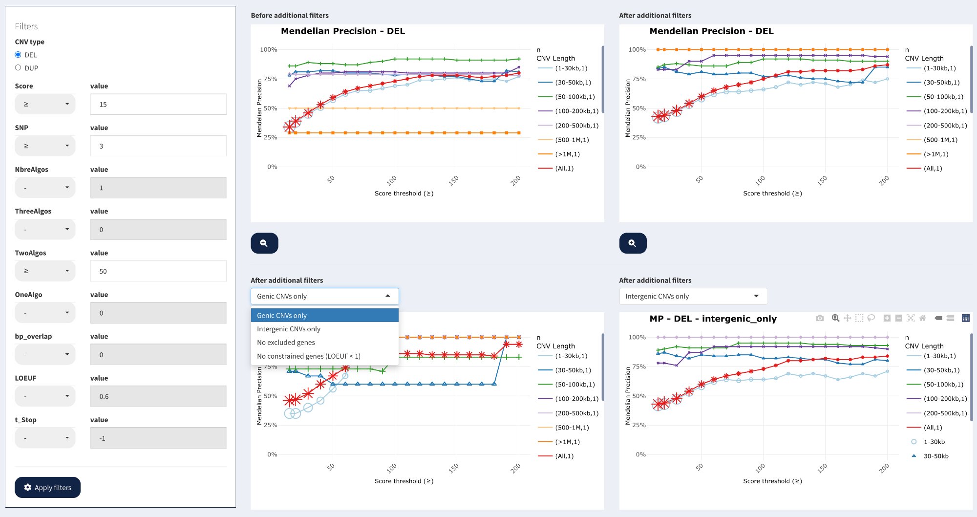
Complete Fine-tuning interface showing CNV filtering criteria (left), four comparative plots (Before / After / Genic / Intergenic), and subset selection dropdown.
The interface consists of:
Left panel: CNV filtering criteria with operators and values
Main area: Four comparative line plots showing MP vs Score threshold
Subset dropdown: Select additional analyses (Genic, Intergenic, No excluded genes, etc.)
CNV type selection
Select the CNV type to analyze:
DEL — Analyze deletions only
DUP — Analyze duplications only
Recommendation: Optimize DEL and DUP separately to identify type-specific thresholds.
CNV filtering criteria
Define filtering criteria using CNV characteristics from your original file plus annotation data added during preprocessing.
Note
Available filters include: (1) columns from your original CNV file, and (2) annotation columns added during the Preprocessing step. The app automatically detects which columns can be used for filtering.
Always available (from Preprocessing annotation):
bp_overlap — Base pair overlap with genes (added by gene annotation)
LOEUF — Gene constraint score (added by gene annotation)
cnv_problematic_region_overlap — Problematic regions overlap (added by annotation)
size — CNV size in bp (calculated during annotation)
Required in your original CNV file:
CHR, START, STOP, TYPE, SAMPLE_ID
Commonly available from your CNV file:
Score — Caller-specific quality score (strongly recommended)
User-specific columns (variable):
Any additional columns in your original CNV file
Custom quality metrics, caller-specific fields, etc.
Operators:
≥ (greater than or equal)
≤ (less than or equal)
= (equal)
- (no filter applied)
Example filtering strategy:
CNV type: DEL
Score ≥ 15                              # From your CNV file (if present)
bp_overlap ≥ 1000                       # From annotation (always available)
LOEUF ≥ 0.6                            # From annotation (always available)
cnv_problematic_region_overlap ≤ 0.5   # From annotation (always available)
Apply filters:
Click Apply filters to generate the comparative plots using the available columns.
Comparative plots
Four plots are displayed to compare MP under different filtering scenarios:
Plot organization:
Top left: Before additional filters (baseline from MP Exploration)
Top right: After additional filters (with quality thresholds applied)
Bottom left: After additional filters + subset analysis (default: Genic CNVs only)
Bottom right: After additional filters + subset analysis (default: Intergenic CNVs only)
Plot features:
X-axis: Score threshold (≥ values)
Y-axis: Mendelian Precision (0-100%)
Multiple lines: One per size range (1-30kb, 30-50kb, …, >1Mb, All)
Variable marker shapes: Marker size represents CNV count at that threshold * Stars, triangles, circles, etc. * Larger markers = More CNVs at that threshold * Smaller markers = Fewer CNVs at that threshold
Interactive: Hover for detailed tooltips
Interpretation:
Before vs After: Compare top-left (baseline) with top-right (filtered) to assess improvement
MP increase: Look for how much MP improves with quality filtering
CNV count: Tooltips show “n” (count) — assess trade-off between quality and quantity
Genic vs Intergenic: Bottom plots reveal if intergenic CNVs have lower quality
Subset analyses
Use the dropdown menu in the bottom plots to select additional subset analyses:
Available subsets:
Genic CNVs only — CNVs overlapping genes
Intergenic CNVs only — CNVs not overlapping any genes
No excluded genes — Exclude CNVs overlapping genes in exclusion list
No constrained genes (LOEUF < 1) — Exclude CNVs in highly constrained genes
Use cases:
Genic vs Intergenic: Identify if intergenic CNVs have systematically lower MP
No excluded genes: Assess impact of excluding specific gene sets
No constrained genes: Estimate technical MP by removing likely true de novo events
Example workflow:
Apply quality filters (e.g., Score ≥15)
Compare “After” plot (all CNVs) vs “No constrained genes” plot
If MP is similar → filters are effective (removing technical false positives)
If MP differs substantially → filters may be removing genuine de novo CNVs in constrained genes
Plot modal (enlarged view)
Click any plot title to open an enlarged modal view:
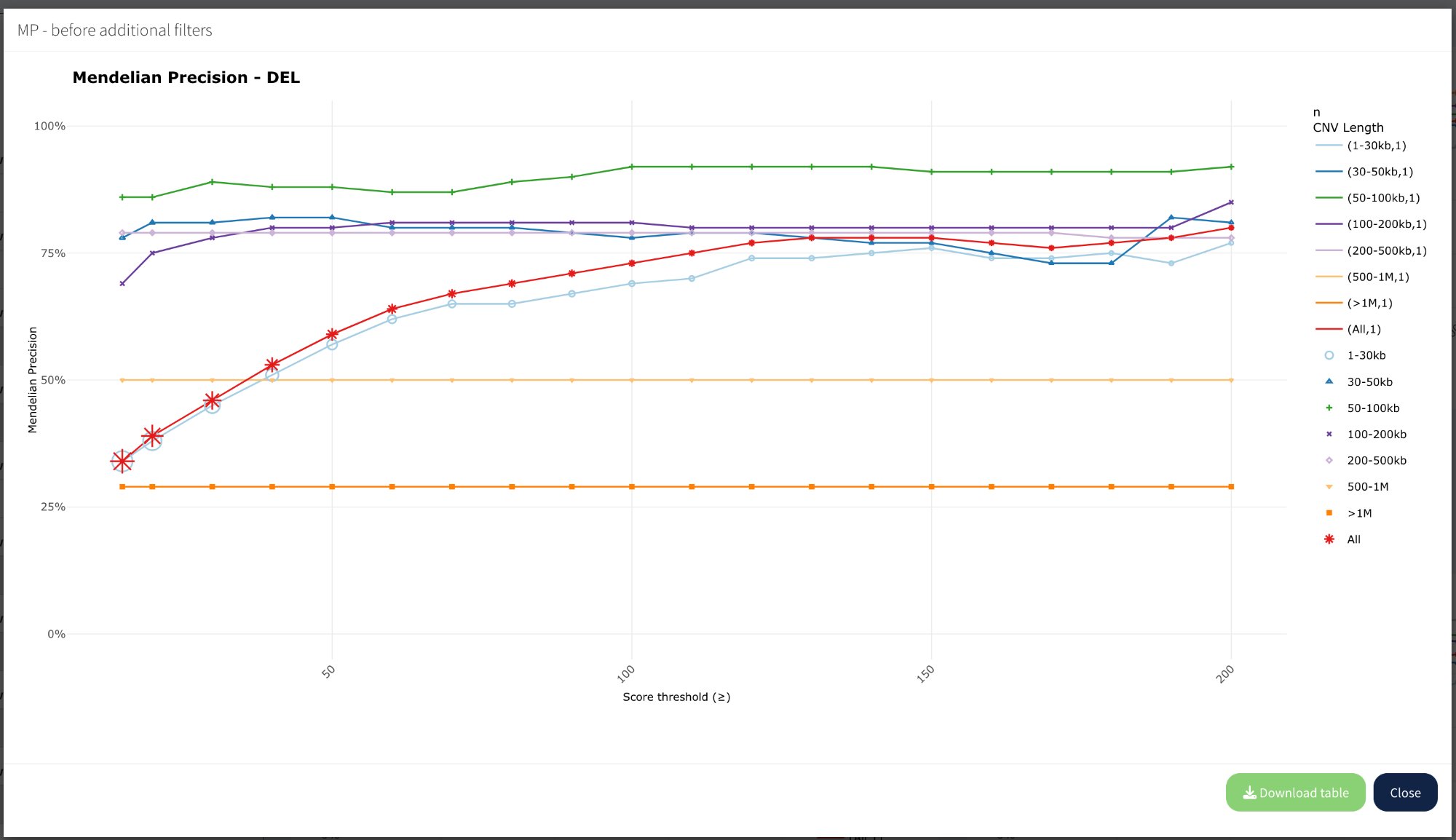
Modal view showing enlarged “MP - before additional filters” plot with full legend, Download table button, and Close button.
Modal features:
Larger plot: Better visibility of lines and trends
Full legend: All size ranges visible on the right
Download table: Export data for this specific plot as CSV
Close button: Return to main Fine-tuning view
Download table:
Click Download table to export the underlying data for the displayed plot. The table includes Score threshold, MP values, and CNV counts for each size range.
Optimal threshold identification
Strategy for finding optimal thresholds:
Start with baseline: Observe “Before” plot MP values
Apply lenient threshold: Set low threshold (e.g., Score ≥10)
Observe improvement: Compare “Before” vs “After” plots
Increase gradually: Incrementally raise threshold (Score ≥15, ≥20, ≥30, etc.)
Identify plateau: Look for point where MP stops improving significantly
Balance trade-off: Choose lowest threshold at plateau to maximize CNV retention
Example decision process:
From the screenshot, for deletions:
Score ≥15:
- "All" line shows MP ~30-70% depending on size
- Small CNVs (1-30kb) still show low MP ~30%
- Large CNVs (50-100kb) show high MP ~90%

Interpretation:
- Score ≥15 is effective for medium-large CNVs
- Small CNVs may require higher thresholds or additional filters
- Consider size-specific thresholds in downstream analyses
What to look for:
Steep slope: MP increasing rapidly → threshold is effective
Plateau region: MP stops improving → increasing threshold further loses CNVs without gain
Size-specific patterns: Different size ranges may plateau at different thresholds
Download filtered tables
Each plot has an associated filtered table that can be downloaded:
Available downloads:
Before filters: Baseline CNV table (from MP Exploration filters only)
After filters: CNV table with quality thresholds applied
Genic only: CNVs overlapping genes
Intergenic only: CNVs not overlapping genes
No excluded genes: CNVs excluding specified gene list
No constrained genes: CNVs excluding LOEUF < threshold
How to download:
Click plot title to open modal
Click Download table button
CSV file is saved to your downloads folder
File format:
Tab-delimited CSV with all CNV columns plus:
Annotation columns (genes, LOEUF, etc.)
Inheritance columns (Transmitted_CNV, Transmitted_gene)
Only CNVs passing the specific filter scenario
Strategy 4: Size-aware filtering
For 1-30kb CNVs: Score ≥ 200
For 30-100kb CNVs: Score ≥ 100
For >100kb CNVs: Score ≥ 50
# Size-specific thresholds (apply offline after download)
See also
Filtering strategies — Detailed filtering strategies
Mendelian Precision — MP calculation methods
Outputs — Output file formats
CLI tutorial — Command-line workflow alternative
Tips and tricks
Efficient filtering workflow
Start broad — Use MP Exploration with minimal filters to assess baseline
Identify issues — Look for size ranges or types with low MP
Optimize systematically — Use Fine-tuning to test quality thresholds
Balance quality vs quantity — Target MP ≥85% while retaining sufficient CNVs
See also
Preprocessing — Preprocessing steps explained
Filtering strategies — Filtering strategies
Outputs — Output formats and interpretation
CLI tutorial — Command-line workflow alternative